Optimizing a Core Model from a Data Sheet

The Jiles-Atherton core model used within Micro-Cap is a model based upon contemporary theories of domain wall bending and translation. There are seven parameters that make up this model. Four of them determine the shape of the B-H curve, and three are based on physical measurements of the core. The four curve fitting parameters need to be optimized in order to produce a reasonable B-H curve for a specific core material. While a manual process of iterating the core model parameters is possible, this can be quite tedious. The simplest method to produce a core model is to use the Model program capabilities that come with Micro-Cap. The Model feature is designed as an interactive, optimizing curve fitter that can take numbers from data sheets and output model parameters for simulation. The Model programming capability in Micro-Cap is invoked by either creating a new MDL file or by opening an existing MDL file. 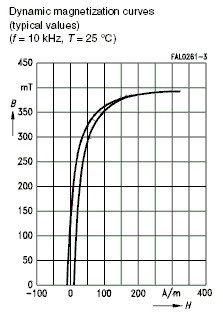This article is going to go through the process of creating a core model of the T35 MnZn core material available from Epcos. The B-H curve at an operating frequency of 10kHz and a temperature of 25C taken from the T35 data sheet is shown below.

Once the B-H curve information is available, the first step is to launch the Model feature within Micro-Cap. Under the File menu, select the New option. Change the type to MDL and click OK. The model may also be added to an existing MDL file. In this case, use the Open command to open the desired MDL file. Next click on the Model / Add Part / Core menu sequence. A new core entry will be created in the file that will be used to input the T35 information. Four text fields in the upper left of the screen, T1 through T4, are available for each part. The T1 field holds the part name. The T3 field holds the memo description of the part. The T2 and T4 fields are comment fields used only within the MDL file. For the T35 model, the fields have been defined as follows: T1: T35 T2: Source - EPCOS SIFERRIT PDF Datasheet T3: Core MnZn Material T4: Spectrum Software 1/12/2005 In the Epcos data sheet, the B-H curve has its units defined in terms of Teslas versus A/m. In the Model file, the core initially has its units defined in terms of Gauss versus Oersted. To toggle between these core unit specifications, select the Change Core Units option under the Model menu. Once the core units match the units used in the data sheet, it is time to input data from the B-H curve. The core takes data triplets as the input. The first two fields are the H value and its corresponding B value. The third field in the triplet is one called Region. The Region will take a value of 1, 2, or 3. A value of 1 designates the B-H data as being part of the initial permeability curve. A value of 2 designates the data as part of the top B-H curve, and a value of 3 designates the data as part of the bottom B-H curve. Typically, when estimating data points from a B-H curve, data should be taken from the top half (B>0) or the right half (H>0) of the curve. Model will create the missing half as a mirror image. Since the Epcos data sheet only displays the top half, the choice in this case is easy. The following data triplets have been estimated from the data sheet and entered into the Model file: H B Region 0 0 1 200 .385 2 35 .3 2 8 .2 2 -10 0 2 10 0 3 28 .2 3 55 .3 3 200 .385 3 Since the initial permeability curve was missing in the Epcos data sheet, only a single triplet was entered for Region 1 where both the H and B values are at 0. Both Region 2 and Region 3 have been represented with four data points each. Typically, each region should contain around four to six data points. With too few data points, the Model optimizer may not have a good enough sample. With too many data points, the Model optimizer may not optimize as closely to the data sheet B-H curve. Although seemingly counterintuitive, this last point is due to the fact that each data point is weighted equally in importance. The Model optimizer tries to find the curve that produces the least amount of error in relation to all of the data so it may create a greater error margin in a crucial area of the curve in order to tighten up the error margin in a less important area of the curve. Once all of the data triplets have been entered, the Area, Path, and Gap parameters can be manually set in the Model Parameters section of the screen. Since the T35 is a core material rather than an actual core component with a geometry, these parameters will be left at their default values in this case. The four curve fitting parameters can now be calculated. Under the Model menu, the Optimize command initiates the optimization. 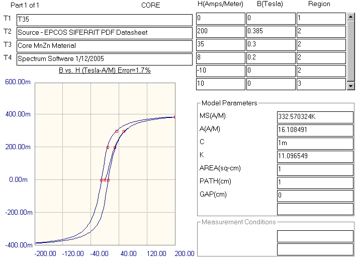The final results of the Model optimization for the T35 model appear below.

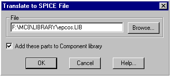
While the T35 optimization process is complete, this model is currently still available only in the MDL file. The next step is to make it accessible to the rest of Micro-Cap by creating a SPICE library file and adding the model to the Component library. This process is done by simply selecting the Add These Parts to the Component Library command under the Model menu. The dialog box that is invoked is shown below.

The File field defines the name and location of the SPICE library to be created. The Add these Parts to the Component Library checkbox will add all of the parts in the MDL file to the Micro-Cap Component library. Generally, this checkbox should be enabled. If disabled, this command will only create the corresponding SPICE library file. Click OK to complete the process. The newly created SPICE library will now be displayed. Both this library and the MDL file may now be closed. The T35 component is now available for placement in a schematic. Since the MDL file was called Epcos.mdl, the T35 component was placed in a group called Epcos on the main level of the Component menu. 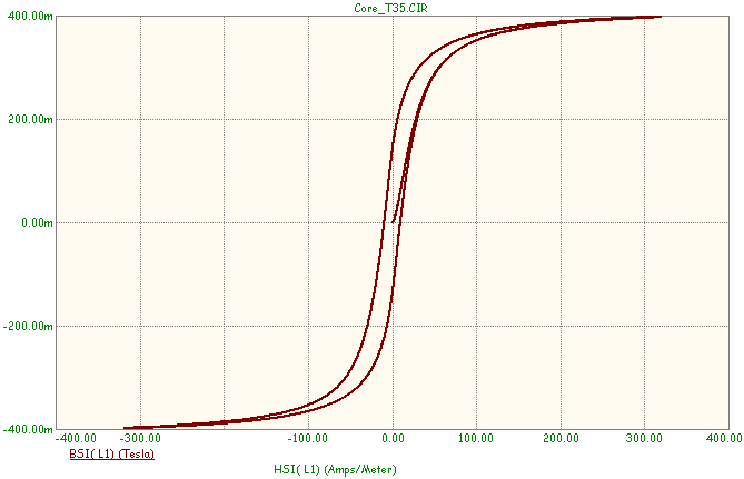The transient analysis displayed below shows the B-H curve of the T35 core model produced during a Micro-Cap simulation. Note that the B and H values of the curve have been plotted using the BSI and HSI operators. These operators produce the B and H values in terms of Teslas and A/m whereas the standard B and H operators will produce Gauss and Oersted.

Return to the main Newsletter page