|
|
 |
Using Performance Functions to Analyze a Filter
Performance functions are mathematical procedures designed to aid in extracting measures of circuit performance from waveforms generated during an analysis. Micro-Cap provides functions to measure performance related values such as rise time, width, peak, valley, high, low, and many others. A useful feature of the performance functions is in creating performance plots. Performance plots may only be used when at least one parameter, including temperature, in the circuit is being stepped. A performance plot is created by plotting one data point from each stepped run that matches the criteria of a specified performance function.
Performance functions are useful for any type of circuit. In the example that follows, a couple of performance functions will be used to aid in the analysis of a filter.
|

|
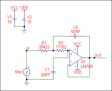
The circuit above is an active Chebyshev filter. This circuit is modified from one available in the FILTER.CIR file. The pulse source 'Filter' provides an AC small signal source of 1 volt magnitude. The opamp LM709 is actually an ideal level 1 opamp model that only models the gain and finite output resistance.
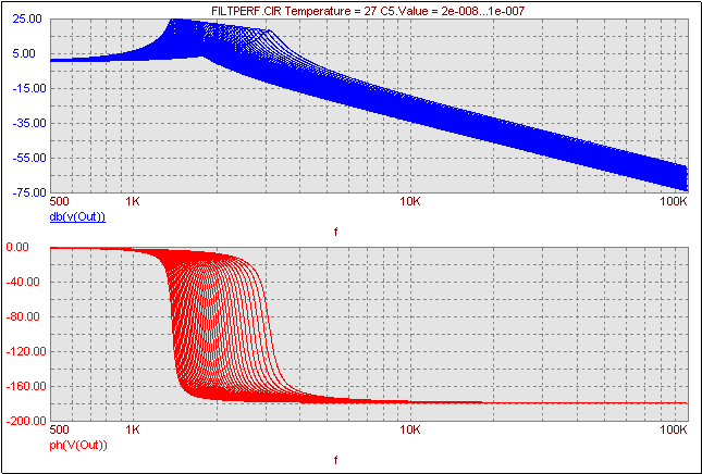
The figure below displays the AC analysis of the gain and phase waveforms at node 'Out'. The feedback capacitor, C5, has been stepped from 20nF to 100nF in steps of 2nF. For increasing values of the feedback capacitor, the bandwidth gets smaller and the ripple gets larger. The bandwidth and the ripple are the two waveform characteristics that will be analyzed through the use of performance plots.
|

|
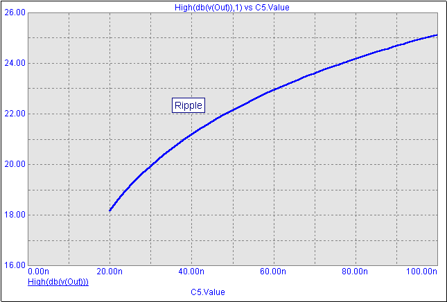
To plot the performance plot of the ripple versus the stepped capacitor, we will use the performance function High on the dB(V(Out)) waveform. The High function finds the global maximum of each stepped run, and then returns the maximum of each run for plotting. The top figure below displays the performance plot of the ripple versus the capacitance of C5. The plot shows the ripple increasing as the capacitor is increased which is as expected. The performance function Peak may also have been used in this case, but since the ripple is the highest data point in the plot, High is easier to use.
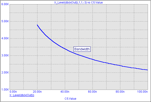
To plot the performance plot of the bandwidth versus the stepped capacitor, we will use the performance function X_Level on the dB(V(Out)) waveform. The X_Level performance function has two parameters, N and Y Level. This function will find the Nth instance of the specified Y Level value, and it will then return the corresponding X value for that expression. In this case, N is specified as 1, and Y Level is specified as -3. Therefore, the first time that the function finds the -3dB level of the gain waveform, it will return the corresponding frequency at which this occurs. This will give us the bandwidth value. The bottom figure displays the performance plot of the bandwidth versus the capacitance of C5. As expected, the bandwidth decreases when the capacitor is increased.
Performance functions may be used on any waveform that is plotted. In the above examples, we could have also used the ph(V(Out)) waveform if that would have provided us with the appropriate information.
|

|

|
|
|
|
|


