Importing data from Excel, MATLAB, or any program that can create a text file
is relatively easy. The steps in the process are these:
1) Run the MATLAB program that creates a table of values and saves it in a text file.
2) Edit an existing User Source data file to have the correct headers.
3) Copy the generated data into the User Source data file from 2). Rename the user source file.
4) In your circuit, add a plot of the User Source data file.
5) Run the Micro-Cap analysis and you'll see a plot of the data from the user file.
Here is an example of the sequence:
1) Run the MATLAB program that creates a table of values and saves it
in a text file.
Here is a MATLAB program that generates a file called mc11_test.txt containing
a table of values T and EXP(T).
% create a matrix y, with two rows
x = 0:0.01:1;
y = [x; exp(x)];
% open a file for writing
fid = fopen('mc11_test.txt', 'w');
% print a title, followed by a blank line
fprintf(fid, 'Time V(OUT)\n\n');
% print values in column order
% two values appear on each row of the file
fprintf(fid, '%f %f\n', y);
fclose(fid);
% create a matrix y, with two rows
x = 0:0.01:1;
y = [x; exp(x)];
% open a file for writing
fid = fopen('mc11_test.txt', 'w');br>
% print column headers, followed by a blank line
fprintf(fid, 'Time V(OUT)\n\n');
% print values in column order
% two values appear on each row of the file
fprintf(fid, '%f %f\n', y);
fclose(fid);
If you run this file in MATLAB it will create the text
file mc11_test.txt, which contains this:
Time V(OUT)
0.000000 1.000000
0.010000 1.010050
0.020000 1.020201
0.030000 1.030455
...
0.970000 2.637944
0.980000 2.664456
0.990000 2.691234
1.000000 2.718282
2) Edit an existing User Source data file to have the correct headers.
Start with any user file (*.usr). For example, here is the Sample.usr file
from the USER.CIR sample circuit file.
[Main]
FileType=USR
Version=2.00
Program=Micro-Cap
[Menu]
;Simple = T,X,Y
;SimpleNoX = T,Y
;Complex = F,Xr,Xi,Yr,Yi
;FormatType = Simple | Complex | SimpleNoX | ComplexNoX
;Format=FormatType
WaveformMenu=label vs T
[Waveform]
Label=label vs T
MainX=T
LabelX=T
LabelY=label vs T
Format=Simple
Data Point Count=256
0,0,0
3.921568627E-009,3.921568627E-009,0
7.843137255E-009,7.843137255E-009,0
1.176470588E-008,1.176470588E-008,0
...
Edit the header so that it looks like the following. You can use any text
editor including Micro-Cap to edit the text.
[Main]
FileType=USR
Version=2.00
Program=Micro-Cap
[Menu]
;ComplexNoX= F,Yr,Yi
;FormatType = Simple | Complex | SimpleNoX | ComplexNoX
;Format=FormatType
WaveformMenu=V(OUT) vs T
[Waveform]
Label=V(OUT) vs T
MainX=T
LabelX=T
LabelY=V(OUT) vs T
Format=SimpleNoX
Data Point Count=102
3) Copy the generated data into the User Source data file from 2).
Rename the user source file.
Here we copy the waveform data from the mc11_test.txt text file and paste
it to the table area of the User Source file from step 2) so that it now
looks like this:
[Main]
FileType=USR
Version=2.00
Program=Micro-Cap
[Menu]
;ComplexNoX= F,Yr,Yi
;FormatType = Simple | Complex | SimpleNoX | ComplexNoX
;Format=FormatType
WaveformMenu=V(OUT) vs T
[Waveform]
Label=V(OUT) vs T
MainX=T
LabelX=T
LabelY=V(OUT) vs T
Format=SimpleNoX
Data Point Count=102
0.000000 1.000000
0.010000 1.010050
0.020000 1.020201
...
0.980000 2.66456
0.990000 2.691234
1.000000 2.718282
Rename the modified user file to something like mc11_test.usr.
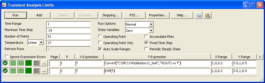
4) In your circuit, add a plot of the User Source data file.
In your circuit, add a plot. Use T in the X Expression field. In the Y expression,
right click in the field and select the Curve option and then the Curve Y option.
Specify the User Source file name and Expression name used in 2). Your analysis
limits should look like this:
Here we have added the plot of EXP(T) for a comparison check:
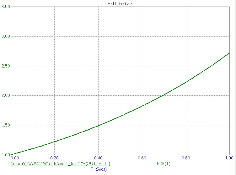
5) Run the Micro-Cap analysis and you'll see a plot of the data from the user file.
Here is what the analysis plot looks like:
|