Correlating Monte Carlo Parameters

A Monte Carlo simulation provides a method to view how the circuit performance can be affected by varying specified circuit parameters. The Monte Carlo simulation performs a number of runs varying the circuit parameters randomly within the tolerances defined in the schematic for each run. This is to ensure that the circuit will behave within acceptable limits while accounting for any possible variation in component values within the tolerance band. Only model parameters and symbolic variables (created through define statements) are available for tolerancing. Both absolute (LOT) and relative (DEV) tolerances are available. Specifying a tolerance for a model parameter is done by including the keywords LOT and/or DEV after the model parameter value. An example of this for the BF parameter in an NPN model would be: .Model N1 NPN (IS=1f BF=300 Lot=30% Dev=5% BR=50) With the standard use of the tolerance specifications, the only correlation between different devices will be between those that reference the same model. The parameter values between devices using the same model will track exactly when just the LOT keyword is specified and the appropriate flag of either the PrivateAnalog or the PrivateDigital option in the Global Settings is disabled. When enabled, the PrivateAnalog and PrivateDigital options force each device to use their own private instance of the model so that no correlation is possible. If the DEV keyword is specified or the corresponding Private option is enabled, each device that references the model will have a unique tolerance value. For the symbolic variables, only the absolute tolerance is available because only one instance of the variable is present. The LOT tolerance in this case is specified before the variable name. An example of tolerancing a variable called RTest would be: .Define {Lot=10%} RTest 50 Since only one instance of the variable is present, all devices that reference the symbolic variable will be correlated. The LOT and DEV keywords have optional syntax that provides an additional means of correlating the tolerance values of devices within a schematic. The full syntax for the LOT and DEV keywords are: LOT[/<lot#>][/<distribution name>] = <value>[%] DEV[/<lot#>][/<distribution name>] = <value>[%] The <lot#> specifies which of ten random number generators, numbered 0 through 9, are used to calculate parameter values. This lets you correlate parameters within an individual model statement as well as parameters between models or symbolic variables. Using the <lot#> lets any toleranced parameter be correlated to any other toleranced parameter simply by sharing the same <lot#> value. The DEV random number generators are distinct from the LOT random number generators. Tolerances without this specification get unique random numbers. The <distribution name> specifies the distribution that will be assigned to the toleranced parameter. It can be defined as Uniform, Gauss, or WCase to define the distribution as equal probability, Gaussian, or worst case. This setting will override the global distribution setting defined within the Monte Carlo Options dialog box for that parameter. A resistor model whose R multiplier is being toleranced can be specified as: .MODEL RMOD RES (R=1 Lot/1/Gauss=10%) This model statement would correlate the R parameter with any other parameter whose <lot#> specification has been assigned the value of 1 and sets the distribution method for this parameter to Gaussian. 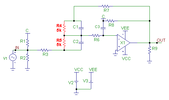An example schematic showing the use of the <lot#> in correlating parameters between model statements is shown below. The schematic models a bass boost circuit where the R4 and R5 resistors simulate a 10kOhm potentiometer. There are numerous ways to model a potentiometer, but in order to display the use of the correlation feature, it will be modelled using just two 5kOhm resistors. The R4 resistor has its Model attribute defined as RMOD1, and the R5 resistor has its Model attribute defined as RMOD2. The two models are stored in the Models text page and are defined as: .MODEL RMOD1 RES (R=1 Lot/1=50%) .MODEL RMOD2 RES (R=1 Lot/1=-50%)

In both models, the R parameter, which is a resistance multiplier, is the parameter that is being toleranced. Since the R parameter is equal to 1 in the models, this technique will tolerance the actual resistance value by the specified percentage for any resistor that references the model. In the LOT keyword specification, the <lot#> entry in both models has been defined as 1. During a Monte Carlo simulation, the R parameter from each model will be correlated with each other. Note that the tolerance percentage for RMOD2 has actually been defined as -50% whereas the tolerance percentage for RMOD1 is 50%. Defining the percentages in this manner will actually set an inverse correlation between the two model parameters. For example, if the R4 resistor is toleranced to produce a resistance value of 5.3kOhm, then the R5 resistor will be toleranced to produce the value of 4.7kOhm. If both tolerances had been set to 50%, then both resistances would have been set at 5.3kOhm. For the R4 and R5 resistors, the inverse correlation means that the series combination resistance of the two will always be equivalent to 10kOhm during any Monte Carlo run. Setting the resistors up in this manner is equivalent to tolerancing the position of the wiper in a 10kOhm potentiometer. 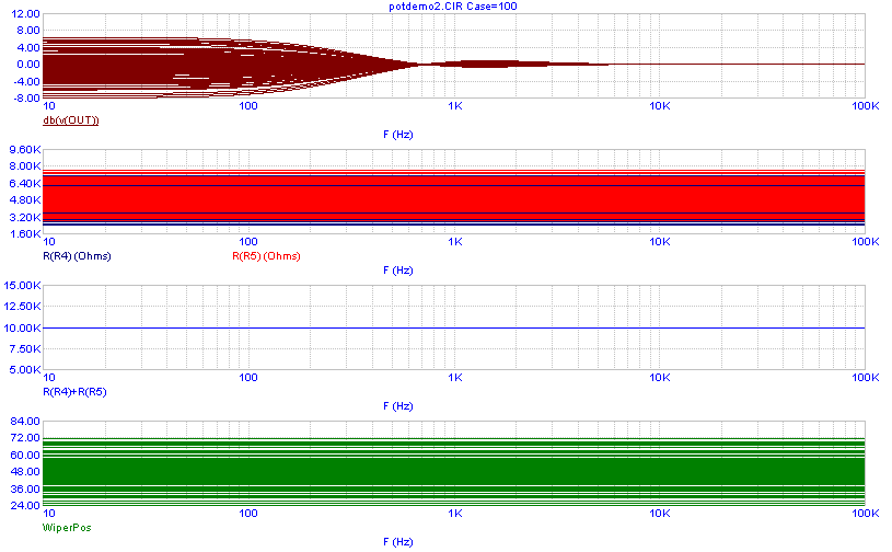The AC analysis results of a Monte Carlo simulation are shown below The Monte Carlo options have been defined to perform a 100 run simulation using a Gaussian distribution.

The first plot displays the output voltage of the bass boost circuit in decibels by plotting the expression dB(V(Out)). The second plot displays the resistance values for both the R4 and the R5 resistor for each of the Monte Carlo runs. The third plot displays the sum of the R4 and R5 resistances during the run. Due to the inverse correlation, the sum of the two resistors always comes out to 10kOhm. The outcome of the simulation is similar to randomly moving the wiper of the potentiometer to a new position and then viewing the resulting frequency response. The fourth plot displays the output of a variable called WiperPos. The WiperPos variable was created with a .Define statement in the schematic whose syntax is: .define WiperPos ((10k-R(R5))/10k)*100 The WiperPos equation will calculate the value of the wiper position in terms of the percentage that the wiper has been moved. At the 0% position, all 10kOhms would be represented by the R5 resistor, and at the 100% position, all 10kOhms would be represented by the R4 resistor. 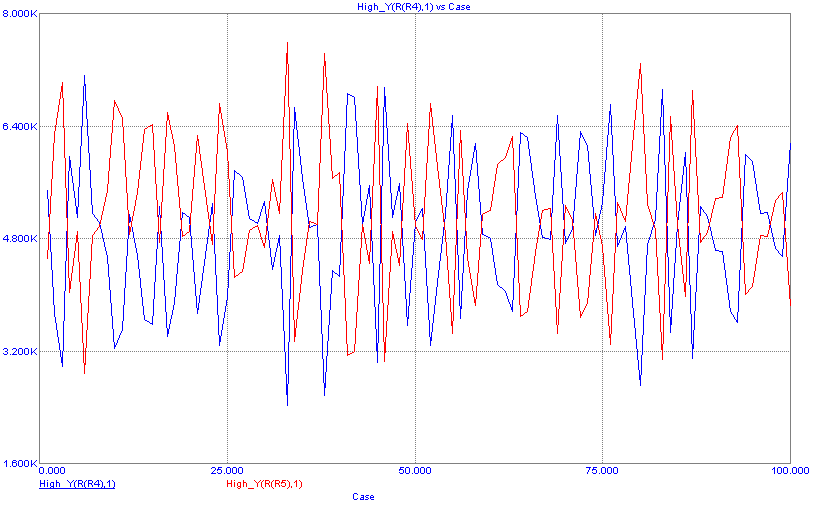A nice way to view the inverse correlation of the R4 and R5 resistances is to create a performance plot from their associated resistance waveforms. The performance plot uses performance functions to harvest a single data point from each branch of the simulation and then creates a plot from the corresponding set of data points. The performance plot created from one Monte Carlo simulation is shown below.

There are two waveforms in the performance plot. The performance functions used to create these waveforms are: High_Y(R(R4),1) High_Y(R(R5),1) The High_Y performance function returns the maximum Y value for the specified waveform for each branch of the Monte Carlo simulation. Since the resistances are constant during each branch, the High_Y function just returns the resistance value for that branch. These waveforms are plotted versus the Monte Carlo branch that each value was calculated from. The inverse correlation between the two resistors can be easily viewed with this plot.

Return to the main Newsletter page