|
|
 |
Table Defined Resistance
The VALUE attribute of the resistor has the capability to be defined with either a constant or an expression. However, not all applications for a resistor can conform to a standard expression. In some cases, a resistor may need to be defined with a table of values. For example, the load of a circuit may need to be varied to simulate the connection of different devices over time. The Table operator in Micro-Cap is available for this situation. The syntax of the Table operator is as follows:
TABLE(x,x1,y1,x2,y2,...xn,yn)
where x is the variable used as the input. This operator returns a value for y associated with the value of x, interpolated from the table. X values less than x1 generate an answer of y1. X values greater than xn generate an answer of yn. The data points must be entered in input ascending order where x1 < x2 < ...xn.
The circuit below displays an example of a resistor using the Table operator. This resistor is used as the load for a lossless transmission line that is defined with a characteristic impedance of 50 ohms and a delay of 100ns. The resistor has its VALUE attribute defined as:
Table(t,0,50,4.9u,50,5.1u,100,9.9u,100,10.1u,150)
|

|
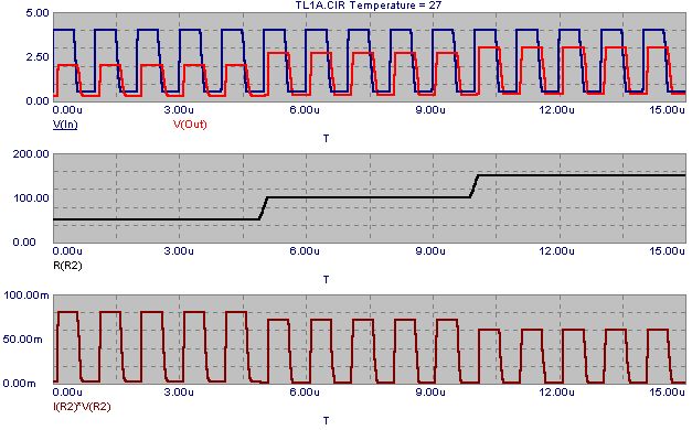
Time has been declared as the input variable. The output of the table is defined where the load resistance will be 50 ohms between 0s and 4.9us, 100 ohms between 5.1us and 9.9us, and 150 ohms from 10.1us on. The time frames of 4.9us to 5.1us and 9.9us to 10.1us are the periods where the resistor linearly transitions to the new value. The input to the transmission line is a pulse source with a 50 ohm series resistance. The pulse source uses the following model statement:
.Model Pulse Pul (Vzero=0.5 Vone=4 P1=5n P2=20n P3=500n P4=600n P5=1000n)
which provides a pulse from .5V to 4V of width 480ns every 1us.
The analysis below displays the transient analysis results of this circuit for a 15us simulation. The top plot is the voltage at both the In and Out nodes. The magnitude of the voltage at node Out is dependent on the load resistance. At 50 ohms, the magnitude is 2V. At 100 ohms, the magnitude is 2.67V. At 150 ohms, the magnitude is 3V. This matches the results obtained by a voltage divider equivalent of this circuit. The middle plot is a plot of the resistance of the resistor R2. As can be seen in the figure, the plot of the resistance matches exactly with the specified data points within the Table operator. The bottom plot of the figure displays the power dissipated in the R2 resistor. The power was plotted with the expression I(R2)*V(R2).
|

|
While this example used a simple time based input, the Table operator can also use dynamic variables such as voltage or current as its input. This allows great flexibility in using this method to create models of switches, thermistors, voltage suppressors, and other resistor varying models. The actual data values for x1,y1 through xn,yn must be constant values when entering an analysis so dynamic variables are not available when defining these.
|
|
|
|
|


