|
|
 |
Monte Carlo Tolerances and Distributions
Several recent requests about the nature of the Monte Carlo LOT and DEV tolerances have prompted us to
include an article on the subject.
In Micro-Cap both absolute (LOT) and relative (DEV) tolerances can
be applied. A LOT tolerance is first applied to each device which uses the same model statement.
A DEV tolerance is then added to the first through last device relative to the LOT toleranced value
originally chosen for the first device. In other words, the first device in the list receives a LOT
tolerance, if one was specified. All devices, including the first, then receive the first device's
value plus or minus the DEV tolerance. DEV tolerances provide a means for having some devices track
in their critical parameter values.
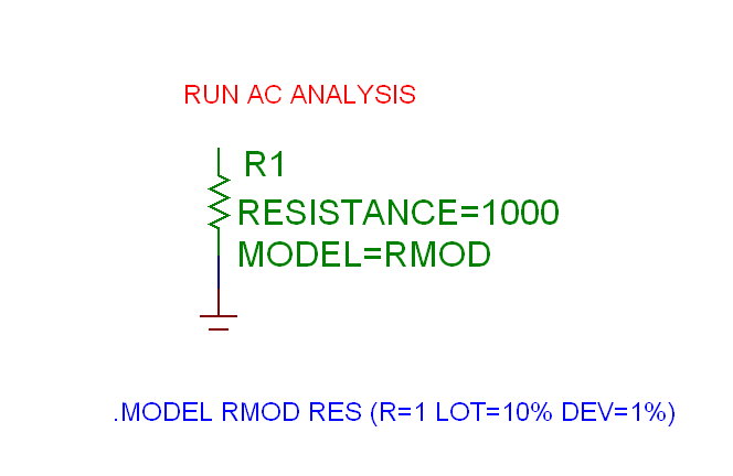
Note that both LOT and DEV tolerances are calculated based on the original value. Let's look
at an example. In the circuit below there is a single resistor R1 whose nominal value is 1000. It
uses the RMOD model statement which looks like this:
.MODEL RMOD RES (R=1 LOT=10% DEV=1%)
The resistor value is 1000*R, where R is the toleranced Resistance Multiplier model parameter.
If the Worst Case distribution is used, all resistor values must be one of these four:
1000*(1+.1+.01) = 1000+100+10 = 1110
1000*(1+.1-.01) = 1000+100-10 = 1090
1000*(1-.1+.01) = 1000-100+10 = 910
1000*(1-.1-.01) = 1000-100-10 = 890
So whether you do 10 runs or 1000 runs all of the values will be chosen from this set of four.
|

|
To illustrate how this works, run AC analysis. Its Analysis Limits dialog box looks like this.
|
Here we're plotting just the resistance of R1. We're using just two data points per run to speed things
up. As the resistance doesn't vary with frequency, what we'll see is a set of horizontal lines whose Y
value equals the resistance computed for that run. Here is what the 40 runs look like.
|
As expected, we see four horizontal lines representing the resistance values of the 40 runs. The reason
there are only four is that using a Worst Case distribution with a LOT and DEV tolerance only four
values are possible. To see this in a Monte Carlo sense, look at the next figure which shows the histogram
and a list of the resistance values.
|
This figure shows the histogram for the 40 runs using a Worst Case distribution. Since there are only four possible values, we get only
four bars. In the list to the right are shown the 40 values used in the Monte Carlo run. As you can see
there are are 40 instances, but only four distinct values. The key point of this simplified example is to
demonstrate how the values are computed and show that they really are computed that way. In most
Monte Carlo situations, one uses a Gaussian distribution. This is how the resistance distribution might
look for a typical run using a Gaussian distribution.
|
|
|
|
|


