|
|
 |
Modeling Skin Effect in an AC Analysis
The lossy transmission line component can now use the F and S variables directly in the model statement of the device. Any of the four
impedance parameters (R, L, C, and G) can use these variables in order to define a frequency dependent expression for an AC analysis
simulation. This capability provides a simple method to model transmission line characteristics such as skin effect.
Skin effect is the phenomenon where the apparent resistance of a wire increases as the frequency increases. At DC, the charge carriers have an
even distribution throughout the area of the wire. However, as the frequency increases, the magnetic field near the center of the wire
increases the local reactance. The charge carriers subsequently move towards the edge of the wire, decreasing the effective area and
increasing the apparent resistance.
The area through which the charge carriers flow is referred to as the skin depth. The skin depth is frequency dependent, and we will use
it to calculate the AC resistance by implementing its transfer function in the R parameter of the lossy transmission line model. The first
step is to compute the transfer function for the AC resistance. The AC and DC resistances are related through the effective area of the wire
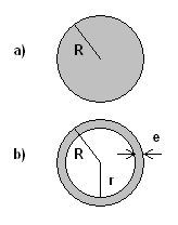
as follows. Refer to the figure below for a graphical representation of the variables used.
AC resistance / DC resistance = DC area / AC area
AC resistance = (DC area / AC area) * DC resistance
DC area = PI * R * R
AC area = (PI * R * R) - (PI * r * r)
r = R - e
e = (3.16e3 / (2 * PI)) * Sqrt(res / (f * km))
AC resistance = ((PI * R * R) / (PI * R * R - PI * (R - e)*(R - e))) * DC resistance
where e is the skin depth, res is the resistivity, f is the frequency, and km is the relative permeability. The AC resistance has now been reduced to
depending on only the frequency variable and constants. The skin depth equation presented here is only valid for higher frequency analysis, so we will
analyze it at 50kHz and higher.
|

|
The basic lossy transmission line model using the skin effect equation is as follows where Rad is the radius of the line, Res is
the resistivity, km is the relative permeability, and DCRes is the DC resistance.
.MODEL TLSkin TRN (C=2n L=1.12n LEN=1
+ R={((PI*Rad**2)/((PI*Rad**2)-PI*(Rad-503.3*(sqrt(Res/(km*F))))**2))*DCRes})
As an example, a pair of 1 meter sections of AWG No. 22 wire will be simulated. Two transmission line models will be created, one
line using copper material characteristics and the other line using aluminum material characteristics. The resulting models are as follows:
* Copper Line
.MODEL TLCopper TRN (C=2n L=1.12n LEN=1
+ R={((PI*.322m**2)/((PI*.322m**2)-PI*(.322m-503.3*(sqrt(1.75e-8/(1*F))))**2))*.0537})
* Aluminum Line
.MODEL TLAlum TRN (C=2n L=1.12n LEN=1
+ R={((PI*.322m**2)/((PI*.322m**2)-PI*(.322m-503.3*(sqrt(2.83e-8/(1*F))))**2))*.0868})
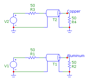
The transmission lines have been setup in the configuration shown below with source and load resistances of 50 ohms.
|

|
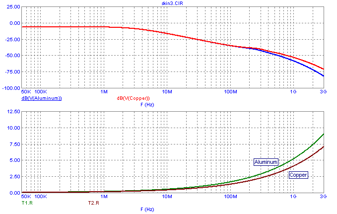
The resulting AC analysis is shown below. The top plot displays the output voltage of each tranmission line in decibels. As can be seen, at higher
frequencies the aluminum transmission line produces a higher AC resistance and a greater loss.
The bottom plot displays the actual resistance value being used for each transmission line in the simulation. The T1.R expression plots the R parameter
for the T1 component which is the aluminum line. The T2.R does the same for the copper line.
|

|
The use of the F and S parameters in the transmission line is only meaningful in an AC analysis. For any other analysis, these variables are set
to a value of 0. For the skin effect model, that would produce a divide by 0 problem. In this case, the transmission line models can be set through
the following If statement.
.if analysis==_AC
.MODEL TLCopper TRN (C=2n L=1.12n LEN=1
+ R={((PI*.322m**2)/((PI*.322m**2)-PI*(.322m-503.3*(sqrt(1.75e-8/(1*F))))**2))*.0537})
.MODEL TLAlum TRN (C=2n L=1.12n LEN=1
+ R={((PI*.322m**2)/((PI*.322m**2)-PI*(.322m-503.3*(sqrt(2.83e-8/(1*F))))**2))*.0868})
.else
.MODEL TLCopper TRN (C=2n L=1.12n LEN=1
+ R={((PI*.322m**2)/((PI*.322m**2)-PI*(.322m-503.3*(sqrt(1.75e-8/(1*Freq))))**2))*.0537})
.MODEL TLAlum TRN (C=2n L=1.12n LEN=1
+ R={((PI*.322m**2)/((PI*.322m**2)-PI*(.322m-503.3*(sqrt(2.83e-8/(1*Freq))))**2))*.0868})
.endif
If the analysis type is AC, then the first pair of models is used. For any other analysis, the second pair of models is used. The only
difference between the two sets is that in the second pair the F variable has been replaced with a variable called Freq. The Freq variable
would need to be set through a define statement such as:
.define Freq 1Meg
In this case, the resistance value of the transmission lines when operating at 1MHz would be used in the other analyses.
|
|
|
|
|


