BJT Temperature Modeling

For many SPICE models, temperature modeling has not been optimized. The temperature parameters that affect the characteristic curves of the model are typically left at their default values which may not be accurate for simulations whose temperature setting deviates from the temperature that the model's parameters were optimized at. Most device models are optimized at either 25 or 27 degrees Celsius which is considered room temperature. The circuit optimizer that is available in transient, AC, or DC analysis for Micro-Cap can be used to derive the temperature parameter values for more accurate simulation results. For the BJT model, the two primary temperature parameters in the model are XTI and XTB. XTI is the saturation current temperature exponent and is used to change the transistor global saturation current sensitivity. The global saturation current is used in the computation of the current through the diodes that connect from the base to the collector and emitter. Modifying XTI generally affects the low current region of the beta curve more than the high current region. XTB defines the temperature coefficient for betas. Modifying XTB vertically shifts the nonlinear beta curve. 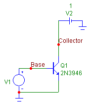The circuit below is used to plot the nonlinear beta curve in transient analysis. The transistor model used in the circuit is a 2N3946 general purpose NPN transistor. The data for this transistor model was derived from the Motorola "Small-Signal Transistors, FETs, and Diodes" data book. In the data book, the VCE for the current gain characteristic is specified at one volt so the battery at the collector in the circuit has been given the same value. The voltage source at the base of the transistor has been defined as follows: DC 0 AC 1 0 Pulse .15 1.5 0 .5 1 .5 5 which will provide a voltage ramp from .15V to 1.5V during the first .5s which is the length of the simulation that will be run.

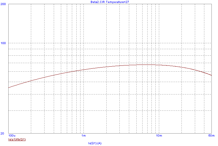
The results of a .5s transient simulation of this schematic when the temperature is set to the nominal temperature of 27C produces the nonlinear beta curve shown below. This curve matches closely with the curve shown in the Motorola data book.

If the Temperature field is set to 100 in the Transient Analysis Limits dialog box, the beta curve that is then produced is a good deal off of the one specified in the data book for that temperature. The reason for this is that the XTI and XTB model parameters are set to their default values. The optimizer available within transient analysis will be used to calculate values for XTI and XTB to better match the beta curve at 100C. Prior to entering the optimizer, the settings in the Transient Analysis Limits dialog box must be set to the values that the curve is to be optimized at. In this case, the Temperature field is set to 100. 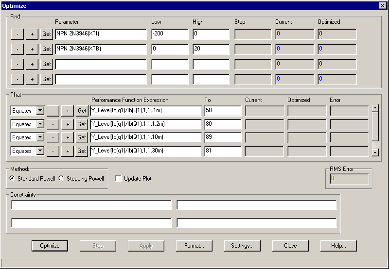To enter the optimizer, select the Optimize option under the Transient menu. For optimizing the XTI and XTB parameters, the optimizer settings for this example are shown below.

The Find section specifies the parameters that are to be optimized. For both the XTI and XTB parameters, the Parameter Type option selected was Model so that the 2N3946 model is being optimized directly. If there was more than one transistor in the schematic referencing the 2N3946 model then all instances of this transistor would be optimized with this option rather than just the single specified transistor that would be optimized using the Component type method. The Parameter Type along with the parameter to be optimized can be selected by clicking on the Get button. Since the object in this optimization is to match the beta curve from the Motorola data book at 100C, the optimizing criteria in the That section for each function is set to Equates. This is the criteria that needs to be used for any curve fitting operation. A sampling of data from the data book for the beta curve at 100C is: @ Ic = .1mA, Beta = 58 @ Ic = 1.2mA, Beta = 80 @ Ic = 10mA, Beta = 89 @ Ic = 30mA, Beta = 81 @ Ic = 50mA, Beta = 70 The equivalent performance functions along with their To values that the optimizer needs to use to match to this data is: Function: Y_Level(Ic(Q1)/Ib(Q1),1,1,.1m)    To: 58 Function: Y_Level(Ic(Q1)/Ib(Q1),1,1,1.2m)    To: 80 Function: Y_Level(Ic(Q1)/Ib(Q1),1,1,10m)    To: 89 Function: Y_Level(Ic(Q1)/Ib(Q1),1,1,30m)    To: 81 Function: Y_Level(Ic(Q1)/Ib(Q1),1,1,50m)    To: 70 The Y_Level operator will try to optimize the Y value of the expression Ic(Q1)/Ib(Q1) at the specified X value to the value set in the To field. Since the X Expression in the Transient Analysis Limits dialog box is set to Ic(Q1), the X value is the collector current of the transistor. For example, with the first expression in the list, when the collector current is .1mA, the optimizer will try to determine the values of XTI and XTB in the 2N3946 model so that the output of the Ic(Q1)/Ib(Q1) expression is equal to 58. Since five performance functions have been specified, the optimizer will find the values of XTI and XTB that produce the curve that creates the smallest total RMS error between the target and actual values at each point. Each of the Equates conditions are weighted equally in terms of importance when optimizing. The Standard Powell optimization method has been selected, and no constraints have been specified. Clicking on the Optimize button initiates the optimization. For these particular settings, the optimizer calculates a value for XTI of -65.051 and a value for XTB of 1.193. The total RMS error for the curve is 2.722 which is a good match. Clicking on the Apply button will update the 2N3946 model in the schematic so that the new XTI and XTB values are used. Applying the updated parameters from the optimizer does not actually overwrite the 2N3946 model in either the Micro-Cap library or in the schematic. Instead, any transistors that were previously referencing the 2N3946 model in the schematic will now be referencing a model called 2N3946_OPT1 which has been placed in the Model page of the schematic. The updated model for the 2N3946 appears as follows: .MODEL 2N3946_OPT1 NPN (IS=0.629196F BF=78.0026 NF=929.132M VAF=100 + IKF=145.824M ISE=985.815F NE=1.74045 BR=105.035M IKR=46.8389 ISC=100P RE=2 + RC=394.919M CJE=7.01663P VJE=907.488M MJE=300M CJC=4.87834P VJC=756.556M + MJC=300M TF=570.088P XTF=500.002M VTF=10 ITF=9.94048M TR=3.50347U + XTB=1.193 XTI=-65.051) This model is a copy of the 2N3946 model with just different values for XTB and XTI. 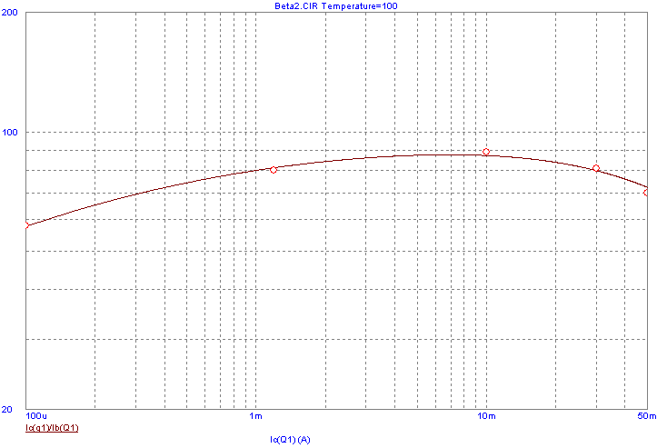Running the same schematic with the updated model statement produces the nonlinear beta curve at a simulation temperature of 100C that is shown below. This beta curve matches closely with the one shown in the Motorola data book.

Return to the main Newsletter page