|
|
 |
Modeling Impedance with Tabular Data in AC Analysis
Quite a few components can be modeled in Micro-Cap by simply simulating their impedance
characteristics. One method to model a complex impedance is to combine resistors, inductors,
and capacitors together until the impedance versus frequency curve matches the expected
results. This method can be very time consuming if done by hand. If the model is to be
simulated in an AC analysis, an easier method is described in this article that will use
data triplets of the frequency, impedance magnitude, and impedance phase to represent the
complex impedance.
One device where modeling the complex impedance is crucial for an AC simulation is a
loudspeaker. A typical speaker will specify a nominal impedance such as eight ohms. This
only describes the standard impedance of the speaker. Over different frequencies, the
speaker impedance may vary drastically from this nominal value. At this point, it will be
assumed that the impedance magnitude and phase versus frequency for the loudspeaker has
already been obtained through measurement of a physical device, from a data sheet, or through
another program. For this example, the impedance curve defines the impedance characteristics
for a fifteen inch, eight ohm loudspeaker from 1Hz to 20kHz. This curve was derived from data
in the book "High Performance Audio Power Amplifiers" by Ben Duncan. Once the data is
available, it should be converted into a .define statement and placed in the Text page of a
schematic. Part of the define statement for the specified loudspeaker is as follows:
| .define Speaker |
| + 1.000000, | 6.642448, | 7.075845 |
| + 1.050764, | 6.648317, | 7.075845 |
| + 1.104105, | 6.654794, | 7.430443 |
| + 1.160153, | 6.661941, | 7.802316 |
| + 1.219047, | 6.669827, | 8.192229 |
| . | . | . |
| . | . | . |
| . | . | . |
| + 16406.252669, | 70.373163, | 85.429172 |
| + 17239.098286, | 73.939376, | 85.649411 |
| + 18114.222406, | 77.689242, | 85.859090 |
| + 19033.771253, | 81.632330, | 86.058708 |
| + 20000.000000, | 85.778745, | 86.248742 |
This define statement creates the symbolic variable Speaker. The + signs are used as a
continuation character to tell Micro-Cap that the following lines are still associated with
the Speaker variable. Each data triplet is defined as:
Frequency, Impedance magnitude, Impedance phase
Alternatively, the real and imaginary values of the impedance can also be used in this
method by defining the triplet as:
Frequency, Real impedance, Imaginary impedance
The components within Micro-Cap that can read in data in this type of format are the Laplace
table sources. The Laplace table source comes in four varieties: LTIofI - current
controlled current source, LTIofV - voltage controlled current source, LTVofV - voltage
controlled voltage source, and LTVofI - current controlled voltage source. For modeling
impedance, only the LTVofI and the LTIofV sources are applicable. Due to the data types
specified in the Speaker define statement, the Laplace source which will be used in this
instance is the LTVofI. This Laplace source measures the current through its input, looks
up the transfer function in the defined table, and produces the resultant voltage output.
For impedance, the source should be wired so that the measured input current is the current
through its own voltage output. This creates the function:
V = I * Table transfer function
where I and V are both assigned to the Laplace source output so that the table transfer
function is the direct equivalent of the complex impedance. This method models the voltage
drop that would exist if the impedance was present in the circuit. Should a LTIofV source
be used instead, the voltage inputs need to be wired to measure the voltage across the
current source output as this method would model the current flow that would exist if the
impedance was present. The table data would also have to be transformed into the
following:
Frequency, 1/Impedance magnitude, - Impedance phase
since the table transfer function should now be the equivalent of the conductance. An
example circuit displaying the use of the LTVofI impedance method is displayed below.
|

|
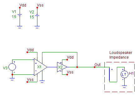
In the schematic, an AC source of magnitude 1 is the input into an INA134 audio differential
line receiver. The output of the INA134 is then fed into the input of a BUF634 high speed
buffer. The Sense pin of the INA134 is connected to the output of the BUF634. This
configuration provides an output current boost to the circuit. The LTVofI component that
models the loudspeaker impedance is connected to the output of the BUF634 device. Note
that the Laplace source has been wired so that it is measuring the current through itself.
The Laplace source has its attributes defined as:
FREQ = Speaker
KEYWORD = Mag Deg
The FREQ attribute defines the table values for the source. In this case, the Speaker
symbolic variable has been entered which will use the define statement that was created
previously and stored in the Text page of the schematic. The KEYWORD attribute defines
the type of data that is specified in the table. Mag indicates that the magnitude value
is true magnitude and Deg specifies that the phase value is in degrees.
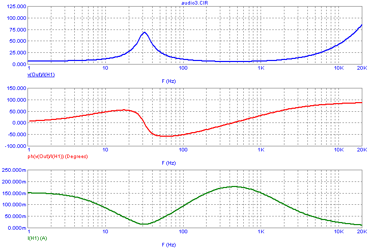
The AC analysis for this circuit is displayed below. The impedance of the speaker output
is calculated by using the expression V(Out)/I(H1). The top plot shows the magnitude of
the impedance and the middle plot shows the phase of the impedance. The impedance curves
show the general impedance characteristics of a loudspeaker. These two waveforms match
precisely with the data that was specified within the Speaker table definition. The bottom
plot displays the output current that is generated through the LTVofI source.
|

|
|
|
|
|


