|
|
 |
Optimizing Subcircuits in the Model Program
The Model program now has the capability to create subcircuits, macros, and other models based on test circuits provided by
the user. This capability provides a method to optimize new libraries of parts using a template model for any type of
component. This article will describe the process of optimizing a subcircuit model for an NTC thermistor in the Model program.
The test circuit in this example is distributed with the professional version of Micro-Cap 10 as SteinHart4.cir.
The first step is to create a subcircuit model that can be used as a template. An NTC thermistor is a thermally sensitive
resistor that adjusts its resistance with changes in temperature in a predictable manner. The behavior of an NTC thermistor can
be modeled accurately through the Steinhart-Hart equation which is as follows:

where

T is the temperature in Kelvin. A, B, and C are the three coefficients that need to be calculated in order to produce an accurate
resistance versus temperature model. The following subcircuit uses .Param statements to define the Steinhart-Hart equation directly
in a resistor component.
.SUBCKT NTC Plus Minus
.PARAM B3C={(B/(3*C))}
.PARAM TK={(TEMP+273.15)}
.PARAM A2={(.5*ALPHA)}
.PARAM ALPHA={((A-1/TK)/C)}
.PARAM TERM1={POW(BETA-A2,.333333)}
.PARAM BETA={SQRT( B3C*B3C*B3C + A2*A2)}
.PARAM A=1M
.PARAM B=100U
.PARAM C=100N
.PARAM RS={EXP( TERM1 - TERM2 )}
.PARAM TERM2={POW(BETA+A2,.33333)}
R1 Plus Minus {RS}
.ENDS NTC
The next step is to create the test circuit that can be used to optimize the circuit parameters. For the Steinhart-Hart equations, the
values that need to be optimized are the A, B, and C parameters. These parameter values can be determined by optimizing the resistance
versus temperature plot of the thermistor.
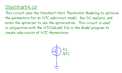
The circuit shown below can be used as the test circuit for the resistance versus temperature curve of the thermistor. The circuit consists
of just a single component that uses the NTC subcircuit model described above. The ground is present because it is mandatory for a ground
node to be present in all schematics.
|
|
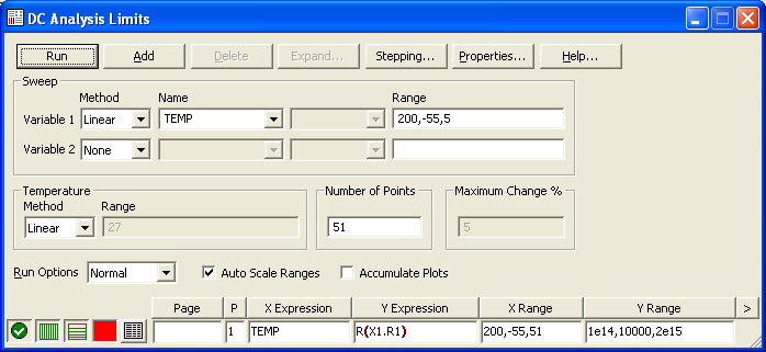
Once the test circuit has been created, the corresponding analysis needs to be setup. For a resistance versus temperature
curve, the best analysis to optimize this in is the DC analysis. The DC Analysis Limits dialog box for the test circuit is
specified as below.
|
|
Temperature is selected as the Variable 1 option and is swept linearly from -55C to 200C. The resistance of the thermistor is plotted
through the Y Expression R(X1.R1). This expression plots the resistance of the R1 resistor that is inside of the X1 component in the
schematic. With the X Expression on that plot line set to the Temp variable, the resistance versus temperature curve of the thermistor
has now been defined.
Once the test circuit has been saved, the NTC subcircuit can be optimized in the Model program. A new model file is created by selecting
New from the Model menu. The New Part dialog box will be invoked automatically which prompts for the device type to specify for the first
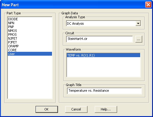
part in the model file. For a user created part, the part type selected should be User. At this point, the Analysis Type, Circuit,
Waveform, and Graph Title can be specified. The Circuit field should be set to the test circuit that was created. Next, the Analysis
Type field is specified as DC Analysis since that was the analysis type used in the test circuit. Once the circuit and analysis type
have been set, a list of available waveforms will be shown in the Waveform field. Only waveforms that have been entered in the analysis
limits of the test circuit will be shown. In this case, the expression TEMP vs. R(X1.R1) is selected. Finally, the Graph Title is
defined as Temperature vs. Resistance. This title simply labels the plot in the Model program. The final settings for the dialog box
are shown below.
|
|
When the OK button is clicked, the model file will be displayed. All of the graph information that was specified in the New Part dialog box can
also be edited in the main model file. The Analysis Type and Circuit fields are available to modify. The waveform can be changed by double
clicking on the header above the graph data, and the graph title can be changed by double clicking on the title above the plot.
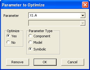
The circuit parameters to be optimized now need to be specified. In the Parameters section, click on the ... button to the right of the top text
field. The Parameter to Optimize dialog box will appear. For the NTC, the A, B, and C parameters set in the .Param statements within the
subcircuit are the objects that need to be optimized. The Parameter Type is set to Symbolic. The Parameter field will then contain a list
of all of the symbolic variables available within the test circuit. The X1.A parameter is selected from this list. The Optimize option
should be set to Yes. The final settings for the dialog box are shown below. When the OK button is clicked, an entry called PARAM X1.A
will now be present in the Parameters section. This same sequence is then repeated for the X1.B and the X1.C parameters on subsequent lines
in the Parameters section.
|
|
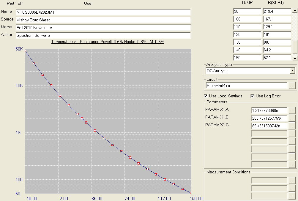
Data to optimize the curve to can now be entered. An NTC thermistor from Vishay with an R25 of 2k ohms is used for this example. The temperature
and resistance pairs are entered in the graph data fields. Since the resistance data spans multiple decades, the Use Log Error option will be
enabled since this typically provides a better fit for logarithmic data. The Optimize command is selected from the Model menu. The final
results of the optimization is shown in the figure below.
|
|
As can be be seen in the plot, the Steinhart-Hart equation provides a very realistic match to the actual datasheet curve. All three
optimization methods used were able to match the curve with an error margin below 1%. When multiple optimization methods are used,
the best match will be shown as the final result. In this case, the best match has an error of 0.5%.
The optimized subcircuit can now be created by selecting the Create Model for this Part command under the Model menu. This command uses the
name specified in the Name field as the name of the subcircuit. There is also an option to add this part to the component library, so you
can immediately place it in a schematic. The subcircuit for the 2k ohm NTC thermistor is as follows:
.SUBCKT NTCS0805E4202JMT Plus Minus
.PARAM B3C={(B/(3*C))}
.PARAM TK={(TEMP+273.15)}
.PARAM A2={(.5*ALPHA)}
.PARAM ALPHA={((A-1/TK)/C)}
.PARAM TERM1={POW(BETA-A2,.333333)}
.PARAM BETA={SQRT( B3C*B3C*B3C + A2*A2)}
.PARAM A=1.3195973068m
.PARAM B=263.7371257759u
.PARAM C=69.4661599742n
.PARAM RS={EXP( TERM1 - TERM2 )}
.PARAM TERM2={POW(BETA+A2,.33333)}
R1 Plus Minus {RS}
.ENDS NTCS0805E4202JMT
If multiple NTC parts were to be created, the current configuration can be saved as a template for easy reuse in optimizing other NTC
models. First, the Name field should be changed to something that describes the generic component. In this case, the Name field could be
set to NTC. Next, select the Save Part to Template Library command under the Model menu. Now when a new part is added to any model file,
NTC will be one of the part type options. It is recommended that the template be stored in its own model file. A new model file could then
be created that would store all the individual instances of the optimized models.
The NTC thermistor is a relatively simple model to setup for optimization. More complex models can also be optimized in the Model program using
multiple test circuits. The Add Graph command under the Model menu, provides a new screen for the model that can use a different test circuit
and optimize other circuit parameters within the model.
|
|
|
|
|


