|
|
 |
Setting a Gaussian Distribution for Random Values
A Gaussian distribution for a random value can be useful for many applications, particularly those in the
communications arena. However, the random functions available within Micro-Cap all have a linear distribution
to them. Fortunately, there is a procedure that can be used to create a Gaussian distributed random expression
from the random functions that already exist in Micro-Cap. (Thanks to Hugh Stevenson for describing this procedure
in the Micro-Cap Yahoo User Group. You can subscribe to the User Group by emailing the
micro-cap-subscribe@yahoogroups.com.)
According to the Central Limit Theorem, linearly distributed random functions can be combined in order to produce
a Gaussian distribution. The Central Limit Theorem consists of the following:
1) The mean of the sampling distribution is equal to the mean of the population from which the samples were
drawn.
2) The variance of the sampling distribution is equal to the variance of the population from which the samples
were drawn divided by the size of the samples.
3) If the original population has a Gaussian distribution, the sampling distribution will also be Gaussian. If
the original population does not have a Gaussian distribution, the sampling distribution will increasingly
approximate a Gaussian distribution as the sample size increases.
The third point is of the most interest in this case. It states that when a number of variables that have
non-Gaussian distributions are combined into a single sample, the distribution of the sample will become
closer to Gaussian distribution as the number of variables used increases. This provides us with the means
to use the linearly distributed random functions to create a Gaussian distribution. Micro-Cap has four functions
which will return a random number between zero and one. The frequency at which a new random number is calculated
is dependent on the function selected as follows:
RND - Returns a new random value every timepoint.
RNDR - Returns a new random value at the start of each Run command.
RNDC - Returns a new random value at the start of each branch of a simulation.
RNDI(t) - Returns a new random value every t seconds of simulation time.
The use of a single one of these random operators produces a linear distribution. Combining two instances of
them will create a triangular distribution. Combining three or more instances of these functions will begin to
produce the familiar bell shape associated with a Gaussian distribution.
Testing this procedure is simple. It only requires a single nonlinear function voltage source (NFV) in
the schematic. For this example, the VALUE attribute of the NFV source has been defined as:
Rndc+Rndc+Rndc+Rndc
Each instance of the RNDC function will return a new random value at the beginning of each branch of a temperature
stepping, parameter stepping, or Monte Carlo run. The RNDC function was selected for the example because it
provides an easy means of creating a histogram that will display the distribution associated with the function
source expression since the value of the defined expression will be constant over the course of a single branch
of a Monte Carlo simulation. Using the RND and RNDI functions in a similar manner would produce a similar
distribution result, although it would be more difficult to display an applicable histogram. Since the RNDR
returns a new random value only at the initiation of the run command, it is not really appropriate for this
method.
The example circuit containing the NFV source is then run through a transient analysis. The Monte Carlo option
is enabled for this simulation. The Number of Runs field in the Monte Carlo options was set to 20000 for the
simulation which will provide 20000 random values created by the function source to test the distribution on.
The Distribution to Use option in the Monte Carlo options was left on Gaussian. This distribution option only
affects parameters that have been toleranced using either the LOT or DEV keywords. It will have no effect on
the distribution of the random functions.
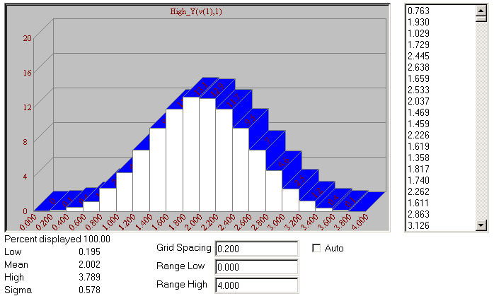
The resulting histogram from the Monte Carlo simulation is displayed below. The histogram was created using
the following performance function:
High_Y(V(1),1)
This performance function selects the highest value from each branch of the V(1) waveform which is the function
source output. Since the function source expression will produce a constant value over a single Monte Carlo
branch, the highest value will just be the value of the expression in the branch. This histogram shows the
results of applying the Central Limit Theorem using the random functions available in Micro-Cap. As can be
seen in the histogram, the distribution has become Gaussian even though all of the random functions in the
expression have a linear distribution.
|

|
In testing this procedure, it appears that a minimum of four instances of the random function is necessary to
produce a reasonable Gaussian distribution. Increasing the number of random function used in the expression
should produce a closer distribution to Gaussian. The histogram below displays the results of summing
eight RNDC functions using the same analysis specifications.
While the range of a single random function is between zero and one, note that the range of the function source
expression in the above examples varies between zero to four and zero to eight depending on the number of random
functions used. In most applications, a scale factor and/or an offset would need to be utilized to compensate
for the use of multiple random functions in the expression.
|
|
|
|
|


